Building custom deep network architectures#
This page is the implementation companion to the theory page, which derives the weight updates, and the prospective configuration tutorial, which walks through a worked classification example. It explains how PyHGF can assemble hybrid models that mix predictive coding networks with custom connectors to replicate wide range of network architectures.
We go through the core DeepNetwork class, the mixed-pipeline machinery
that builds larger models, and the general recipe for porting any architecture.

The main idea#
PyHGF networks are made of nodes that hold beliefs and require a specific belief propagation dynamic to learn (which is the core of PyHGF’s machinery). The DeepNetwork class supports the creation of fully connected multi-layer perceptrons (MLPs). But for users interested in alternative network architectures, this would require adapting this (and adjusting the propagation machinery), which is possible but rapidly limits the expressivity and modularity of the toolbox.
Instead, here, we show how we can keep the main MLP structures in predictive coding form while plugging other components to connect them through fixed transformations. Many neural architectures are indeed merely adding complex transformations around fully connected layers where weight learning is taking place, and because we have these structures available in other frameworks like Equinox or PyTorch, it is rather straightforward to borrow these connectors and plug them into mixed predictive coding architectures.
A DeepNetwork: layers of beliefs#
How to build one??#
import jax
import optax
from pyhgf.model import DeepNetwork

net = (
    DeepNetwork()
    .add_layer(size=8)                              # output layer (bottom)
    .add_layer(size=16, coupling_fn=jax.nn.gelu)    # hidden layer
    .add_layer(size=8)                              # input layer (top)
)
Three conventions to know:
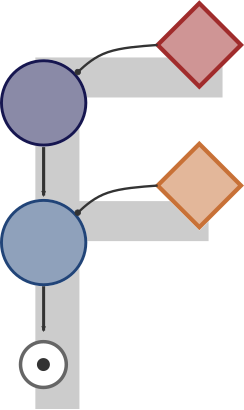
Input on top, output at the bottom. Layer 0 is the output layer (where observations are clamped); the last layer added is the input layer (where predictors are clamped). Predictions flow downward.
The nonlinearity belongs to the predicting layer. A layer’s
coupling_fnis applied when that layer predicts the one below it. The network above therefore computesW1 @ gelu(W2 @ x + b2) + b1— exactly a standardLinear → GELU → Linearblock, with the hidden nodes holding the pre-activation values.Biases are constant nodes. Each layer can carry an always-on constant node (
add_constant_input=True, the default); the bias lives as an extra column of the weight matrix, added linearly.
The three learning steps#
One learning step is three passes over the layers:
Prediction — clamp the input
xon the top layer; every layer predicts the one below it, top to bottom.Update — clamp the observation
yon the bottom layer; compute prediction errors and correct every belief, bottom to top, each correction weighted by confidence.Learning — nudge every weight from its local prediction error and the activity on its other side.
Two ways to feed data#
As a time series (net.fit(x, y, ...)): samples are scanned one at a
time, and the confidences carry over — each prediction reads the previous
posterior precision, so the network’s confidence adapts as the series
unfolds. This is PyHGF’s native filtering mode.
As a batch (net.batch_update(x, y, ...)): samples are exchangeable
(e.g. token positions), so every sample is processed from the same state —
same weights, same confidences — in parallel, and the per-sample updates are
averaged and applied once. The batch counts as a single observation, which
makes the step invariant to repeating the batch.
net.batch_update(
    x_batch, y_batch,                # (batch, n_features) each
    optimiser=optax.adam(3e-3),      # any optax optimiser, applied locally
    update_precisions=False,         # True: confidences also adapt per batch
)
net.input_errors                     # (batch, n_input) — error at the input,
                                     # for whatever sits behind this network
Two flags control what learns: optimiser=None freezes the weights;
update_precisions=False freezes the confidences (used whenever an exact
comparison against backpropagation is wanted). net.input_errors is the
confidence-weighted prediction error routed back to the input layer.
Mixed pipelines: assembling bigger models#
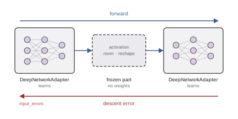
Learning parts (DeepNetworkAdapter around a DeepNetwork) alternate with frozen parts, which hold no weights. Forward, each part computes its output from its input; backward, it receives the descent error at its output, learns from it if it has weights, and hands the error at its input to the part behind it — for a DeepNetworkAdapter, the negated net.input_errors.
Large models are built from parts (pyhgf.model.hybrid). The part
objects declare the model — which slots learn, which are frozen, how they
nest — and every part contributes the same two things to the compiled
training step:
forward: compute my output from my input;
backward: receive the error at my output, learn from it if I have weights, and hand the error at my input to the part behind me.
The arrays passed between parts are descent errors — the gradient of the loss with respect to that signal, the same object a backprop library would hand around.
Two kinds of parts exist:
Learning parts —
DeepNetworkAdapter(net, optimiser=...)wraps aDeepNetwork. It is the single place where the pipeline’s error convention meets PyHGF’s (observed-minus-predicted) convention: the error enters by clampingoutput − erroras the observation the network should have produced, and leaves as the negatedinput_errors.Frozen parts — fixed calculations with nothing to learn, which only translate errors using a hand-derived formula (no autodiff).
Running a pipeline: one compiled program per step#
The part objects only declare the model; FusedPipeline
(pyhgf.model.fused) runs it. Each training step — the forward walk, the
error at the output, every part’s local learning step — is staged into a
single compiled program, so nothing crosses a compilation boundary
inside a step and the per-sample forward states are already in hand when
each part’s update needs them. Usage:
from pyhgf.model import FusedPipeline

pipeline = FusedPipeline(model, lambda probs, ids: probs - jax.nn.one_hot(ids, vocab))
for x, y in batches:
    output, input_error = pipeline.step(x, y)   # one compiled call
probs = pipeline.predict(x_eval)                # forward pass only
pipeline.merge()   # write the trained state back onto the part objects
The error_fn given at construction forms the descent error at the output
inside the program; when omitted,
it defaults to output - target, the squared-error gradient. predict
runs the forward pass alone, for evaluation and generation. The part
objects do not advance while the executor runs; merge() writes the held
state back onto them for inspection or checkpointing.
The general recipe to port any architecture#
Any feed-forward deep learning model can map onto a mixed pipeline with two rules.
Every weight matrix becomes a small PyHGF network. The
pyhgf.model.transplantconverters build them directly from trained (or freshly initialised) Equinox layers, weights carried across so both sides compute the identical function.Weightless calculations become frozen parts. Activations, normalisations, reshapes: each needs only a hand-derived backward formula, verified in tests against autodiff of the same forward.
System configuration#
%load_ext watermark
%watermark -n -u -v -iv -w -p pyhgf,jax,jaxlib
Last updated: Fri, 11 Sep 2026

Python implementation: CPython
Python version       : 3.12.14
IPython version      : 9.16.1

pyhgf : 0.3.2
jax   : 0.6.2
jaxlib: 0.6.2

IPython: 9.16.1

Watermark: 2.6.0