Learning in deep predictive coding networks: the theory#
Backpropagation has underpinned the optimisation of deep networks for decades. It comes with uncontestable advantages, effectively fuelling the development of modern AI, but still has downsides, such as interference during training, catastrophic forgetting, or poor biological realism, which in turn has shaped the development of hardware.
Predictive coding (PC) is the go-to alternative and has proved efficient in tasks typically faced by biological organisms [Song et al., 2024], in which the error back-propagation algorithm can be seen as a special case [Whittington and Bogacz, 2019]. But it has also been historically neglected by the deep learning community as usually slower to train and difficult to scale to deep architectures.
In some sense, PyHGF belongs to the PC lineage, while being slightly non-traditional in its objectives (initially solving inference from sequential data) and in its implementation (closed-form variational updates to find relaxation points instead of iterative gradient descent). This has a main advantage: the training time wall effectively vanishes, and predictive coding networks such as the ones handled by PyHGF can be advantageously applied to discrimination tasks in deep and wide architectures [Baskakovs et al., 2026]. What makes them unusual is how they learn: using a combination of belief updating, precision-weighted prediction error propagation, and Hebbian weight learning. But similarly, in these networks, error backpropagation is found to be a special case of the network parametrisation.
In this section, we expose the theory and differentiate PyHGF from traditional backpropagation and other predictive coding architectures, assuming no prior familiarity with PyHGF, predictive coding, or the mathematics of learning. We cover 1. how deep networks normally learn, 2. how a predictive-coding network learns instead, 3. the theorem saying when the two coincide and its proof, 4. the regimes where predictive coding does something genuinely different, and 5. where PyHGF sits on that map.
Several companion pages complete the picture of this chapter: the DeepNetwork implementation page shows how these ideas become code, the prospective configuration tutorial walks through a worked classification example, and concrete implementations of convolutional networks and transformers are demonstrated afterwards.

Backpropagation: learning in deep neural networks#
A deep network is a stack of neural layers. Each layer holds a vector of activations (numbers describing what the layer currently represents) and is connected to the next by a matrix of weights, the adjustable parameters that the network learns. Data \(x\) enter at one end, are transformed layer by layer (each layer multiplies by its weights and applies a nonlinearity), and a prediction \(\hat{y}\) comes out the other end. A loss function measures how wrong that prediction is compared to an observed outcome \(y\).
Training the neural network means adjusting every weight to make the loss smaller. The central tool is the gradient: for each weight, the derivative of the loss with respect to that weight (i.e., how much and in which direction the loss would change if the weight moved a little). Gradient descent repeatedly nudges every weight a small step against its gradient.
Note
In the rest of this document, we use the PyHGF bottom-up approach of network creation, meaning that we index layers by \(\ell\), with layer \(0\) being the output (\(y\)) and \(\ell\) growing toward the input (\(x\)). We write \(\mu_\ell\) and \(\hat{\mu}_\ell\) for the forward and backward activations of layer \(\ell\), \(W_\ell\) for the matrix of weights connecting layer \(\ell+1\) to layer \(\ell\), and \(g\) for the nonlinearity (a bias is folded into \(W_\ell\) as an always-on constant input).
The forward pass computes, layer by layer,
The hat on \(\hat{\mu}_\ell\) marking a predicted / computed quantity. For an input \(x\), a target \(y\), and the standard squared error, the loss is
with \(f(x)\) the network’s output.
The gradients themselves come from backpropagation: an application of the calculus chain rule that sweeps backward through the network. An early weight affects the loss only through everything downstream of it, so its gradient is a long product of “how each layer affects the next”; backpropagation assembles those products efficiently by introducing, for each layer, an error vector
computed from the output backwards:
where \(g'\) is the derivative of the nonlinearity, \(\odot\) multiplies entry by entry, and \(W_\ell^\top\) is the transpose of the weight matrix. Once the errors are known, each weight’s gradient is an outer product, the error at the layer below times the activity at the layer above:
Backpropagation has a single activation per layer, the forward-pass value \(\hat{\mu}_{\ell+1}\), so both the slope \(g'\) and the activity \(g\) are read there. Predictive coding will have two values to choose between, and which one enters where is what §3 turns on.
Predictive coding#
Predictive coding (PC) is a different way to organise the same computation, drawn from theoretical neuroscience. Instead of activations, each layer holds beliefs: a belief is a guess (a mean, written \(\mu\)) plus a confidence in that guess (a precision, written \(\pi\), the inverse of a variance). Each layer predicts the layer below it through the very same forward map (1), with \(g\) now read as the coupling function. The mismatch between what a layer predicted and what it observed is the prediction error
Important
Backpropagation and predictive coding often use opposite definitions of error terms. \(\varepsilon\) (PC) follows the observed − predicted convention, while \(\delta\) (backpropagation) follows the predicted - observed convention. So, at a clamped output with unit precision \(\varepsilon_0 = y - f(x) = -\delta_0\).
This notation is more natural for PC networks, as the precision-weighted error is what is used to update beliefs at the higher layer (see the theory notebook). When building hybrid architectures (see the next tutorial), the sign of the error is automatically reverted when crossing boundaries between PC networks and handwritten backpropagation components.
The whole network is scored by one quantity, the variational free energy \(F\) for Gaussian beliefs, simply the sum of every layer’s squared prediction error weighted by the precision of that prediction:
The constant absorbs a \(-\tfrac{1}{2}\sum_\ell \log \hat{\pi}_\ell\) term, which is genuinely constant only while the precisions are fixed parameters. The precision here is the predicted one, \(\hat{\pi}_\ell\), because it is the precision of the prediction against which the residual is measured.
A precise layer (high \(\hat{\pi}_\ell\)) is penalised more for the same error, so it “insists” on its predictions; an imprecise layer tolerates mismatch. Learning happens in two nested motions, both descending this same \(F\):
Beliefs settle. Clamp the observation on the output layer (fix \(\mu_0 = y\); a clamped observation is just a belief that is not allowed to move), hold the weights fixed, and let every interior belief slide down the free energy, \(\dot{\mu}_\ell = -\partial F / \partial \mu_\ell\). Each belief is pulled toward its own top-down prediction and pushed by the prediction error of the layer below, gated by the local slope of \(g\). In the textbook variant this relaxation runs for many iterations, until the beliefs reach an equilibrium.
Weights nudge. Each connection then adjusts from purely local quantities, the precision-weighted error on one side $\( e_\ell := \hat{\pi}_\ell\,(\mu_\ell - \hat{\mu}_\ell) = \hat{\pi}_\ell\,\varepsilon_\ell \)\( and the activity on the other: \)\( \Delta W_\ell \;\propto\; e_\ell \; g(\mu_{\ell+1})^\top \)$
This weight rule is Hebbian (“cells that fire together wire together”): the update to a connection is a product of the two quantities available at its two ends. Nothing in it sweeps backward through the network; no part ever sees the whole model. That locality is the point of predictive coding.
Closed-form predictive coding with hierarchical Gaussian filtering#
In [Baskakovs et al., 2026] we introduced an alternative way to build and update similar PC coding networks built on top of hierarchical Gaussian filtering (HGF) machinery, which replaces the iterative relaxation step with closed-form updates (predict once, correct each belief once, nudge the weights once) using the exact update equations of the generalised HGF [Weber et al., 2026].
In this language, the layer above is the value parent of the layer below: the parent’s belief generates the child’s prediction. When a child layer \(\ell\) produces a prediction error, its parent \(\ell+1\) updates its belief using only three things it already has: its own prediction, the connection \(W_\ell\), and the child’s error.
Note
The HGF is initially designed for time-resolved latent state inference, which requires prediction to be made from the previous state position. But here, applying this principle to iterations in a set of predictor-outcome pairs would be meaningless, as the previous label should not influence the current prediction. Therefore, the DeepNetwork class uses a modified update equation that only relies on the expectations (which only come from the parents), instead of the previous mean.
First, the child packages its prediction error together with its own confidence into the precision-weighted prediction error it sends upward:
The parent then updates its precision, adding a “bottom-up” contribution routed through the connection. Writing \(j\) for a node of the parent layer \(\ell+1\) and \(i\) for a node of the fully-connected child layer \(\ell\),
Second, the parent updates its mean by taking a step, sized by one over its posterior precision, in the direction of the routed child error:
Two features of this equation carry the whole of §3. The step is divided by the posterior precision \(\pi_{\ell+1}\) from (2), not by the prior confidence \(\hat{\pi}_{\ell+1}\). And the slope is read at the expected mean \(\hat{\mu}_{\ell+1}\), the parent’s own prediction, exactly as in the precision update above: the posterior mean the equation solves for never enters the slope, which is also what makes the update explicit rather than implicit in \(\mu_{\ell+1}\).
Note
Evaluating the coupling derivatives at the prediction is a property of the volatile layers a DeepNetwork is built from (pyhgf.updates.vectorised.volatile.posterior), where the prediction is the natural reference point because each iteration is an independent predictor-outcome pair. The continuous layers used for time series filtering read them at the posterior mean instead: the previous posterior mean under the standard update, the freshly written one under the eHGF update, which updates the mean first.
When predictive coding equals backpropagation#
There is a specific, well-understood point in the landscape of predictive-coding models where PC weight updates recover BP. The existence of this point has actually been a central argument in favor of PC, but it is crucial to understand that PC can have a range of behaviours around that point that makes it genuinely more interesting.
In this section, we state the condition, prove the equivalence, and illustrate it numerically.
A silent interior#
Predictive coding reproduces exactly backpropagation’s gradients when two things hold: the interior is silent, and every interior layer relays the routed error at full strength rather than attenuating it. We call silent interior the behaviour of hidden activities when they stay at their forward-pass values even after the observation arrives at the output: \(\mu_\ell \approx \hat{\mu}_\ell\), up to a shift that vanishes as the interior precision grows.
When the interior is silent (i.e., when the activation of the forward pass matches the activation of the backward pass), the only effective prediction error in the network is at the output. Every interior layer merely relays the forward pass, and each connection’s local update (error on one side) × (activity on the other) is precisely the chain-rule gradient. If instead the hidden layers moved to satisfy the target, their errors would no longer be backpropagation’s errors, and the two would diverge.
In the classical settling formulation, where precisions are fixed parameters, the silent interior is the whole condition [Whittington and Bogacz, 2017, Millidge et al., 2020]. In the HGF, precisions themselves can be updated and reflect activation uncertainty. Therefore, error is more likely to propagate following a BP gradient in a network made of confident activations, but as errors appear, and as we are logging this uncertainty, the gradient of learning will diverge from BP.
It is therefore straightforward to recover the BP gradient by pinning neurons’ precision to some high number, and disregarding any precision update. This is a way to learn efficiently using local updates and PyHGF PyHGF-only backend, but it is also a more limited way.
Definition 1 (Silent interior)
The interior of a network is silent when every hidden belief stays at its forward-pass value once the observation arrives at the output, \(\mu_\ell \approx \hat{\mu}_\ell\), up to a displacement that vanishes as the interior precision grows. Silent does not mean frozen: the interior still shifts by an infinitesimal amount, just enough to carry the gradient onward. The movement is just too small to change what the activations represent, but is never literally zero.
Definition 2 (Pinning)
An interior layer is pinned when its posterior precision is held at its prior (predicted) value, \(\pi_\ell = \hat{\pi}_\ell\), so the bottom-up contribution of (2) is never written. Pinning to a large value additionally keeps the layer silent (Definition 1).
In code: build the hidden and input layers with
add_layer(..., precision=1e4, expected_precision=1e4), unit precision on the
observed output layer, and fit with update_precisions=False.
Theorem 1 (Pinned single-sweep predictive coding reproduces backpropagation)
Run the single belief propagation with every interior precision pinned to a large constant (Definition 2). Clamping the target seeds the output with the negative loss gradient, \(e_0 = y - f(x) = -\delta_0\) for a squared-error output, \(\text{one-hot} - \text{softmax}\) for a categorical head; the same sign, since \(\partial L / \partial(\text{logits}) = \text{softmax} - \text{one-hot}\). Then the upward messages obey
which is exactly backpropagation’s error recursion (BP). The recursion preserves sign, so by induction down the stack \(e_\ell = -\delta_\ell\) at every layer. Pinning to a large constant additionally keeps the interior silent (Definition 1), so the activity entering the Hebbian outer product converges to its forward-pass value and the local weight step is the backpropagation descent step, node for node:
The proof: the precision ratio \(r\)#
Goal. Rewrite the HGF mean update as a recursion in the upward messages \(e_\ell\), compare it line for line with backpropagation, and close the gaps between the two. The whole argument turns on one quantity:
Definition 3 (Precision ratio)
The ratio of a layer’s prior (predicted) to posterior precision,
\(r_\ell\) is a per-unit quantity, one ratio per node, not a single number per layer. It is at most \(1\), and pinning precisions sets \(r_\ell = 1\) exactly.
Proof. Step 1: read off the parent’s own residual. The parent’s residual is just its displacement from its prediction. Subtract \(\hat{\mu}_{\ell+1}\) from both sides of (3):
Step 2: form the parent’s own upward message. By the definition of the upward message, the parent’s message to its parent is \(e_{\ell+1} = \hat{\pi}_{\ell+1}\,\varepsilon_{\ell+1}\). Multiply (4) by \(\hat{\pi}_{\ell+1}\):
The gain in front is exactly the precision ratio of Definition 3.
Step 3: compare with backpropagation. Put (HGF) next to (BP):
The two routes are now identical; they thread the error through the same matrix and read the slope at the same point, the forward-pass value \(\hat{\mu}_{\ell+1}\). Only two discrepancies separate the recursions:
The per-unit gain \(r_{\ell+1}\le 1\) that hierarchical Gaussian filtering applies at each step and backpropagation does not. This is a byproduct of the Bayesian filtering mechanism that reflects how much nodes are allowed to move under prediction error. Backpropagation does not support this.
The Hebbian outer product that supports the weight updates multiplies the message by the posterior activity \(g(\mu_{\ell+1})\), whereas backpropagation’s gradient \(\partial L / \partial W_\ell = \delta_\ell\, g(\hat{\mu}_{\ell+1})^\top\) reads the activity at the forward-pass value. This is the main mechanism behind prospective configuration.
The exact error backpropagation can therefore be recovered by mitigating these discrepancies. (1) is removed by setting \(r_{\ell+1}=1\), which we can obtain by fixing precision and expected precision to identical values and by removing the precision update so they don’t diverge over time. (2) is mitigated by having a difference between the mean (backward pass) and the expected mean (forward pass) as small as possible (\(\mu_{\ell+1} \simeq \hat{\mu}_{\ell+1}\)). The parent moves by an amount divided by its (large) posterior precision. Make the interior precisions huge, then
A very confident layer barely moves off its prediction, with an error converging to \(0\). The precision-weighted learning update then restores the full gradient by multiplying this error again by the posterior precision. When the precision and expected precision are constants, this effectively recovers the precision ratio \(r_{\ell+1}=\hat{\pi}_{\ell+1}/\pi_{\ell+1}\).
Hint
Is it just backpropagation?
This proof shows that under some restricted conditions, Bayesian filtering in a deep neural
network and weight updates derived from prospective configuration coincide exactly with error
backpropagation. PyHGF’s mean update’s division by the pinned precision and the precision_weighted
weight gradient’s multiplication by it (pyhgf.updates.vectorised.learning) produces
the same reverse-mode vector–Jacobian product jax.grad would build.
The notable difference is that PyHGF never differentiates a graph; it reaches those numbers by local message passing on a generative model. The equivalence is a coincidence of two derivations (variational inference on one side, the chain rule on the other), and it holds only when precisions equal expected precision and when they are set to high values.
The equivalence itself is established in prior work: that silent-interior predictive coding reproduces backpropagation is the theorem of Whittington and Bogacz [2017], made exact on multilayer perceptrons by Song et al. [2020], shown to approximate backpropagation along arbitrary computation graphs by Millidge et al. [2020], and made exact on any computation graph by Salvatori et al. [2021].
What is specific here is the route to it: the equivalence is expressed through the hierarchical Gaussian filter’s own confidence (precision) machinery, and it is reached in a single sweep rather than the settle-to-equilibrium loop. Relaxing this condition will produce largely different behaviours, prospective configuration, which is argued to reduce interference between updates and to help online and continual learning. The two are not in conflict; they are the two ends of one axis, and the precision ratio \(r = \hat{\pi}/\pi\) is that axis’s coordinate. The open challenge for this family of deep predictive coding networks is therefore to find how to settle in the right configuration depending on the learning context.
Where PyHGF sits#
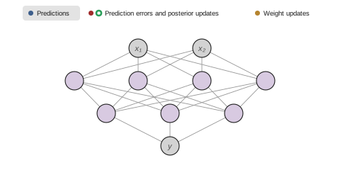
The three passes of a single step. Predictions flow from the clamped predictors \(x\) down to the output \(y\); prediction errors then travel back up, each layer’s posterior being revised as its error arrives; finally every weight is nudged by its own amount. The input layer is clamped, so it carries no posterior update of its own.
PyHGF is single-sweep predictive coding — predict once, correct beliefs once, nudge weights once per batch — with the confidence machinery kept explicit throughout. There is one regime where PC provably learns in fewer steps than backpropagation: faster saddle-to-saddle escape in deeper-than-wide networks. Deep networks trained from a small initialisation descend the loss in a staircase — long flat plateaus (saddle points, where the gradient nearly vanishes and training crawls) punctuated by sudden drops. Because PC learns on the rescaled loss \(L / s(\theta)\), its gradient carries an extra term that is nonzero even where the plain loss is flat, so it slides off those plateaus sooner: the degenerate, slow-to-escape saddles of the loss become benign in the rescaled energy [Innocenti et al., 2024].
Exploring these behaviours means leaving the silent regime on purpose.** Prospective configuration, faster adaptation, and interference resistance all live at the moving-interior end. Reaching it needs three things the current scheme lacks: released precisions (letting \(r\) drop below \(1\), so the interior can move), a settling loop (so it relaxes to an equilibrium instead of taking one sweep), and non-stationary or continual tasks (where the benefit would show).
System configuration#
%load_ext watermark
%watermark -n -u -v -iv -w -p pyhgf,jax,jaxlib
Last updated: Fri, 11 Sep 2026

Python implementation: CPython
Python version       : 3.12.14
IPython version      : 9.16.1

pyhgf : 0.3.2
jax   : 0.6.2
jaxlib: 0.6.2

IPython: 9.16.1

Watermark: 2.6.0