Modelling win-frequency bias in the Iowa Gambling Task

Authors

• Aleksandrs Baskakovs, Aarhus University, Denmark (aleks@mgmt.au.dk)

• Nicolas Legrand, Aarhus University, Denmark (nicolas.legrand@cas.au.dk)

This notebook provides a step-by-step implementation of an HGF-based computational cognitive model for the Iowa Gambling Task, with a specific focus on modelling the win-frequency bias.

import arviz as az
import jax
import jax.numpy as jnp
import matplotlib.pyplot as plt
import numpy as np
import pandas as pd
import pymc as pm
import seaborn as sns
from jax import vmap
from pytensor import wrap_jax
from scipy.special import softmax

from pyhgf.math import binary_surprise
from pyhgf.model import Network
from pyhgf.utils import beliefs_propagation

jax.config.update("jax_enable_x64", True)  # this is required for the softmax

plt.rcParams["figure.constrained_layout.use"] = True

Simulating data

Below we simulate the data for the four decks according to the reward dynamics described in [Ahn et al., 2014].

Deck 1

Deck 1, one of the disadvantageous decks, has a baseline reward of 100 but has a high likelihood (50%) of also containing a punishment of -150 to -350. This means that in 50% of the cases, the total reward will be 100 and in the other 50% of cases it will be 100 - (150 to 350).

num_trials = 100

# set default value to 100.0
deck1 = np.ones(num_trials) * 100.0

# 50% chance to add something between -150 and -350
deck1 += np.random.choice(
    [-150, -175, -200, -225, -250, -275, -300, -325, -350], size=num_trials
) * np.random.binomial(1, 0.5, num_trials)

print(f"Total value of Deck 1: {deck1.sum()}")

Total value of Deck 1: -2425.0

Deck 2

Deck 2, the other disadvantageous deck, has a baseline reward of 100 and a low likelihood (10%) of a high loss of -1250. This means that in 90% of the cases the total reward will be 100 and in 10% of the cases it will be 100 - 1250.

# set default value to 100.0
deck2 = np.ones(num_trials) * 100.0

# 50% chance to add something between -150 and -350
deck2 += -1250.0 * np.random.binomial(1, 0.1, num_trials)

print(f"Total value of Deck 2: {deck2.sum()}")

Total value of Deck 2: -5000.0

Deck 3

Deck 3 is one of the advantageous decks and has the same structure as Deck 1, but with a baseline reward of 50 and 50% likelihood of a punishment of -25 to -75. Even though its baseline reward is lower than that of Deck 1, it has a higher total value due to the lower punishment magnitude.

# set default value to 100.0
deck3 = np.ones(num_trials) * 50.0

# 50% chance to add something between -150 and -350
deck3 += np.random.choice([-25, -50, -75], size=num_trials) * np.random.binomial(
    1, 0.5, num_trials
)

print(f"Total value of Deck 3: {deck3.sum()}")

Total value of Deck 3: 2250.0

Deck 4

Deck 4 is the other advantageous deck, which mirrors the structure of Deck 2, but with a baseline reward of 50 and a 10% likelihood of a punishment of -250. Again, even though its baseline reward is lower than that of Deck 2, it has a higher total value due to the lower punishment magnitude.

# set default value to 100.0
deck4 = np.ones(num_trials) * 50.0

# 50% chance to add something between -150 and -350
deck4 += -250 * np.random.binomial(1, 0.1, num_trials)

print(f"Total value of Deck 4: {deck4.sum()}")

Total value of Deck 4: 3250.0

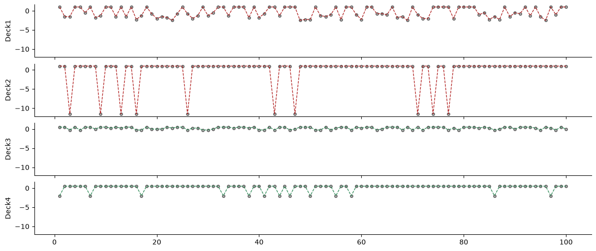
Below, we combine the decks into a list, scale the values and plot the time series of the rewards for each deck.

# Turning the above code into a single function
def generate_decks(num_trials):
    """Simulate a dataset."""
    # Set a random seed for reproducibility
    np.random.seed(77)

    # set default value to 100.0
    deck1 = np.ones(num_trials) * 100.0

    # 50% chance to add a value between -150 and -350
    deck1 += np.random.choice(
        [-150, -175, -200, -225, -250, -275, -300, -325, -350], size=num_trials
    ) * np.random.binomial(1, 0.5, num_trials)

    print(f"Total value of Deck 1: {deck1.sum()}")

    # set default value to 100.0
    deck2 = np.ones(num_trials) * 100.0

    # 10% chance to add -1250
    deck2 += -1250.0 * np.random.binomial(1, 0.1, num_trials)

    print(f"Total value of Deck 2: {deck2.sum()}")

    # set default value to 100.0
    deck3 = np.ones(num_trials) * 50.0

    # 50% chance to add a value between -25 and -75
    deck3 += np.random.choice([-25, -50, -75], size=num_trials) * np.random.binomial(
        1, 0.5, num_trials
    )

    print(f"Total value of Deck 3: {deck3.sum()}")

    # set default value to 100.0
    deck4 = np.ones(num_trials) * 50.0

    # 50% chance to add -250
    deck4 += -250 * np.random.binomial(1, 0.1, num_trials)

    print(f"Total value of Deck 4: {deck4.sum()}")

    decks = [deck1, deck2, deck3, deck4]

    # Scale the decks down by 4
    decks = [deck / 100 for deck in decks]

    return decks

num_trials = 100
decks = generate_decks(num_trials=num_trials)

Total value of Deck 1: -3875.0
Total value of Deck 2: -2500.0
Total value of Deck 3: 2350.0
Total value of Deck 4: 1750.0

# Visualize the decks

# the HGF trials start at 1 - 0 being the prior
trials = np.arange(num_trials) + 1

_, axs = plt.subplots(figsize=(12, 5), nrows=4, sharex=True, sharey=True)

for i, u, label, color in zip(
    range(4),
    [decks[0], decks[1], decks[2], decks[3]],
    ["Deck1", "Deck2", "Deck3", "Deck4"],
    ["firebrick", "firebrick", "seagreen", "seagreen"],
):
    axs[i].scatter(
        trials, u, label="outcomes", alpha=0.6, s=15, color="gray", edgecolor="k"
    )
    axs[i].plot(trials, u, "--", color=color, linewidth=1)
    axs[i].set_ylabel(label)
sns.despine();
# Save the plot
# plt.savefig("plots/decks.png")

Building the model

Now we build a model with 4 HGFs, one for each deck. Every HGF will have the same structure - the continuous input nodes have a value parent - the x1 node, which in turn has its own value parent - x2 node. The x1 nodes will have the autoconnection_strength parameter, which will model the agent’s bias towards decks with high reward frequency.

Perceptual model

autoconnection_strength = 0.2
tonic_volatility = -1.0

# Continuous-state nodes that receive inputs
two_levels_continuous_hgf = (
    Network().add_nodes(
        kind="continuous-state", n_nodes=4, precision=5.0
    )  # replaces "continuous-input"
)

# Value parents for each of the 4 lower nodes
for child in range(4):
    two_levels_continuous_hgf = two_levels_continuous_hgf.add_nodes(
        kind="continuous-state",
        value_children=child,
        precision=5.0,
        mean=1.0,
        tonic_volatility=tonic_volatility,
        autoconnection_strength=autoconnection_strength,
    )

# Value parents for the value parents (stacked hierarchy)
for parent_idx in range(4, 8):
    two_levels_continuous_hgf = two_levels_continuous_hgf.add_nodes(
        kind="continuous-state",
        value_children=parent_idx,
        precision=1.0,
    )

# Visualize network structure
two_levels_continuous_hgf.plot_network()

# Make our input vector - time x branches
u = np.array(decks).T

# Let's feed our hgf the data
two_levels_continuous_hgf.input_data(input_data=u);

if autoconnection_strength == 0.1:
    autoconnection_strength_str = "low"
else:
    autoconnection_strength_str = "high"

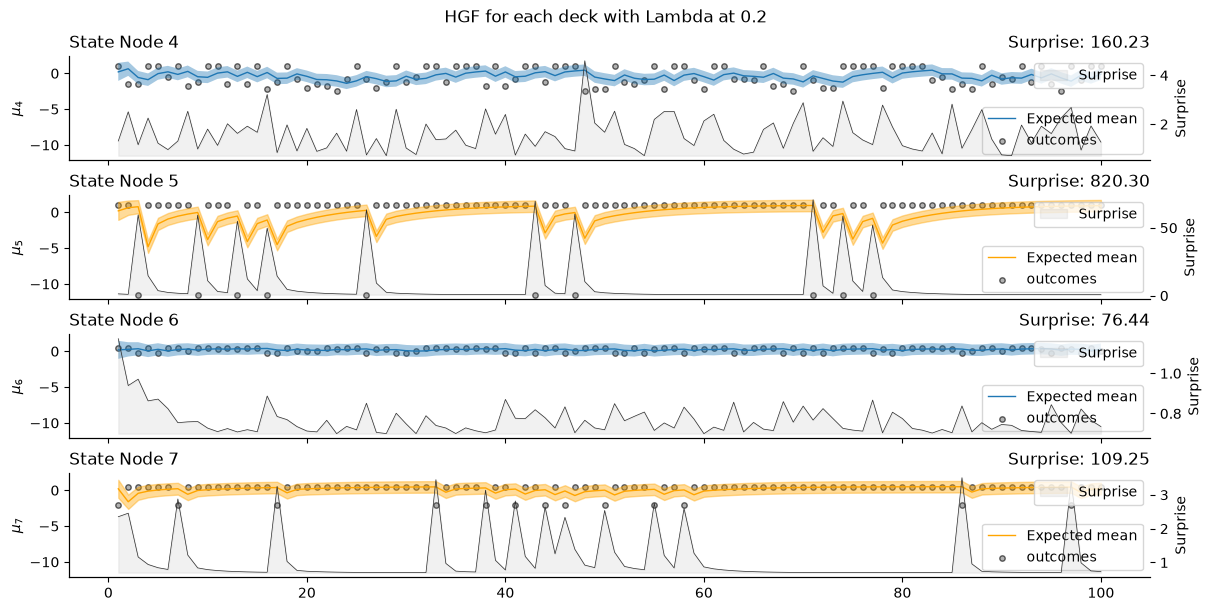
_, axs = plt.subplots(figsize=(12, 6), nrows=4, sharex=True, sharey=True)

two_levels_continuous_hgf.plot_nodes(node_idxs=4, axs=axs[0])
two_levels_continuous_hgf.plot_nodes(node_idxs=5, axs=axs[1], color="orange")
two_levels_continuous_hgf.plot_nodes(node_idxs=6, axs=axs[2])
two_levels_continuous_hgf.plot_nodes(node_idxs=7, axs=axs[3], color="orange")

for i, p, label, color in zip(
    range(4),
    [decks[0], decks[1], decks[2], decks[3]],
    ["Deck 1", "Deck 2", "Deck 3", "Deck 4"],
    ["firebrick", "firebrick", "seagreen", "seagreen"],
):
    axs[i].scatter(
        trials, p, label="outcomes", alpha=0.6, s=15, color="grey", edgecolor="k"
    )
    axs[i].legend(loc="lower right")
# Save the plot
# Add a title to the plot
plt.suptitle(f"HGF for each deck with Lambda at {autoconnection_strength}")
# plt.savefig(f"plots/hgf_nodes_{autoconnection_strength_str}_lambda.png")
sns.despine();

Response model

This section simulates participant decisions in the Iowa Gambling Task (IGT) using the response model:

1. Parameters:

   • beta_1 and beta_2 are inverse temperature parameters set to 1, controlling the influence of expected values and precision on decisions.

2. Extracting Beliefs:

   • means: Expected values for each deck.

   • precisions: Confidence in these beliefs, derived from the model’s precision.

3. Decision Probabilities:

   • A softmax function combines means and precisions to compute the probability of selecting each deck.

4. Simulating Choices:

   • Participant choices are simulated using np.random.multinomial based on the calculated probabilities.

5. Observation Filtering:

   • Only outcomes from the selected deck are observed and stored in observed.

# Simulating choices for the participant
beta_1, beta_2 = 1, 1

means = jnp.array([
    two_levels_continuous_hgf.node_trajectories[i]["expected_mean"] for i in range(4, 8)
])
precisions = jnp.array([
    1 / two_levels_continuous_hgf.node_trajectories[i]["expected_precision"]
    for i in range(4, 8)
])

decision_probabilities = softmax(beta_1 * means + beta_2 * precisions, axis=0)

decisions = np.array([
    np.random.multinomial(n=1, pvals=decision_probabilities[:, i])
    for i in range(decision_probabilities.shape[1])
]).T

# The participants can only see values from the branch they explored
observed = decisions

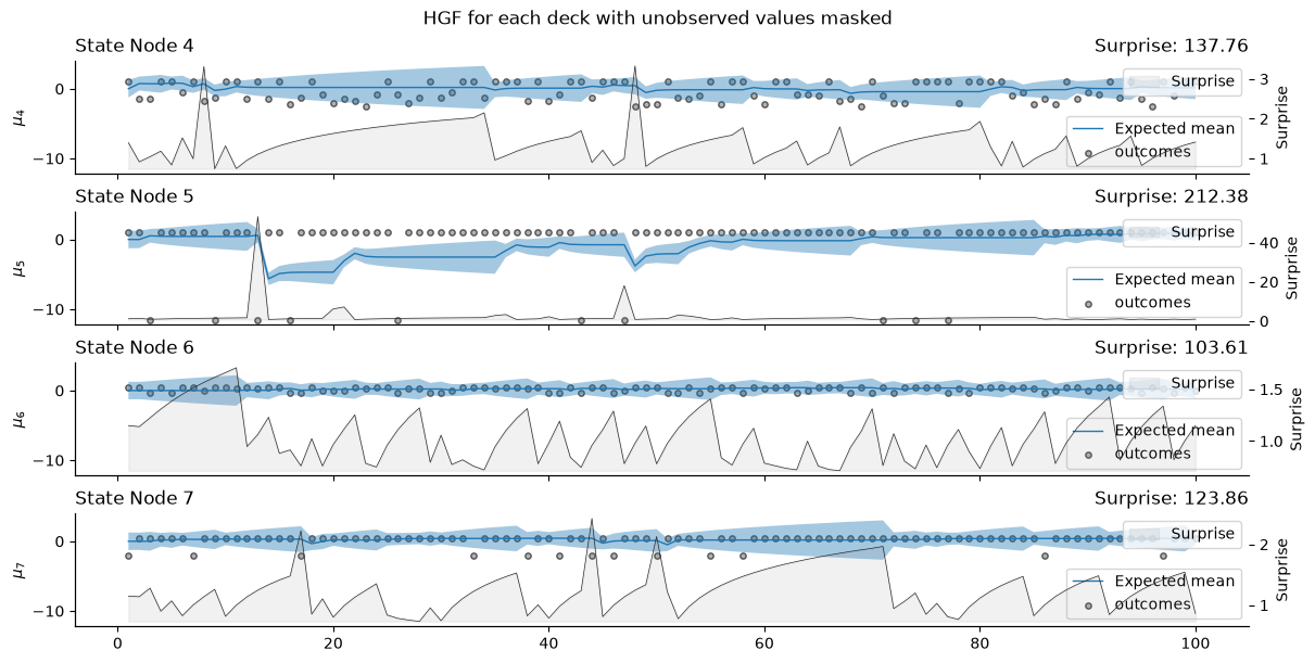
Masking non-selected decks

In the Iowa Gambling Task (IGT), participants only receive feedback on the selected deck. This section simulates that constraint:

• Feedback Mechanism:

  • During each trial, the model updates beliefs using feedback solely from the chosen deck.

  • Inputs for non-selected decks are masked and remain hidden, simulating the real task conditions.

• Belief Updates:

  • For the selected deck, the model processes the feedback to update beliefs.

  • For non-selected decks, the Gaussian Random Walk continues in the background, but the precision of belief updates diminishes due to the lack of new observations.

# Re-initialize the model
two_levels_continuous_hgf = (
    Network().add_nodes(
        kind="continuous-state", n_nodes=4, precision=5.0
    )  # replaces "continuous-input"
)

# Add value parents with relevant autoconnection strength
for child in range(4):
    two_levels_continuous_hgf = two_levels_continuous_hgf.add_nodes(
        kind="continuous-state",
        value_children=child,
        tonic_volatility=tonic_volatility,
        precision=5.0,
        mean=0.0,  # same as before
        autoconnection_strength=autoconnection_strength,
    )

# Add value parents to the value parents
for parent_idx in range(4, 8):
    two_levels_continuous_hgf = two_levels_continuous_hgf.add_nodes(
        kind="continuous-state",
        value_children=parent_idx,
        precision=1.0,
    )

# masking the unobserved values (this step is optional as we are already ignoring them in the observed mask)
# using NaNs will cause intermediate updates to fail so we set the input to arbitrarily high values instead
u[~observed.T.astype(bool)] = 1e6

# note that we are providing the mask as parameter of the input function
two_levels_continuous_hgf.input_data(
    input_data=u,
    observed=observed.T,
);

_, axs = plt.subplots(figsize=(12, 6), nrows=4, sharex=True, sharey=True)

two_levels_continuous_hgf.plot_nodes(node_idxs=4, axs=axs[0])
two_levels_continuous_hgf.plot_nodes(node_idxs=5, axs=axs[1])
two_levels_continuous_hgf.plot_nodes(node_idxs=6, axs=axs[2])
two_levels_continuous_hgf.plot_nodes(node_idxs=7, axs=axs[3])

for i, p, label, color in zip(
    range(4),
    [decks[0], decks[1], decks[2], decks[3]],
    ["Deck 1", "Deck 2", "Deck 3", "Deck 4"],
    ["firebrick", "firebrick", "seagreen", "seagreen"],
):
    axs[i].scatter(
        trials, p, label="outcomes", alpha=0.6, s=15, color="gray", edgecolor="k"
    )
    axs[i].legend(loc="lower right")
# Save the plot
# Add a title to the plot
plt.suptitle(f"HGF for each deck with unobserved values masked")
# plt.savefig(f"plots/hgf_nodes_masked.png")
sns.despine();

Parameter recovery

# Regenerate the decks
num_trials = 100
decks = generate_decks(num_trials=num_trials)

# Create the u vector
u = np.array(decks).T

Total value of Deck 1: -3875.0
Total value of Deck 2: -2500.0
Total value of Deck 3: 2350.0
Total value of Deck 4: 1750.0

# Re-initialize the model
two_levels_continuous_hgf = Network().add_nodes(
    kind="continuous-state", n_nodes=4, precision=5.0
)

# Value parents for each of the 4 lower nodes
for child in range(4):
    two_levels_continuous_hgf = two_levels_continuous_hgf.add_nodes(
        kind="continuous-state",
        value_children=child,
        tonic_volatility=tonic_volatility,
        precision=5.0,
        mean=0.0,
        autoconnection_strength=autoconnection_strength,
    )

# Parents of those parents (indices 4..7)
for parent_idx in range(4, 8):
    two_levels_continuous_hgf = two_levels_continuous_hgf.add_nodes(
        kind="continuous-state",
        value_children=parent_idx,
        precision=1.0,
    )


two_levels_continuous_hgf = two_levels_continuous_hgf.create_belief_propagation_fn()

two_levels_continuous_hgf.plot_network()

attributes, edges, update_sequence = two_levels_continuous_hgf.get_network()

Process the data sequentially, updating the model’s beliefs and parameters based on each decision:

responses = []
means_list = []
variances_list = []

# for each observation
for i in range(u.shape[0]):
    # the time elapsed between two trials - defaults to 1
    time_steps = np.ones(1)

    # the expectations about the outcomes
    mean_1 = attributes[4]["expected_mean"]
    mean_2 = attributes[5]["expected_mean"]
    mean_3 = attributes[6]["expected_mean"]
    mean_4 = attributes[7]["expected_mean"]

    var_1 = 1 / attributes[4]["expected_precision"]
    var_2 = 1 / attributes[5]["expected_precision"]
    var_3 = 1 / attributes[6]["expected_precision"]
    var_4 = 1 / attributes[7]["expected_precision"]

    means = jnp.asarray([mean_1, mean_2, mean_3, mean_4]).ravel()
    variances = jnp.asarray([var_1, var_2, var_3, var_4]).ravel()

    means_list.append(means)
    variances_list.append(variances)

    # compute the softmax
    decision_probabilities = softmax(beta_1 * means + beta_2 * variances, axis=0)
    decision_probabilities = np.asarray(decision_probabilities, dtype=float).ravel()

    response = np.random.multinomial(n=1, pvals=decision_probabilities)

    observed = response

    responses.append(response)

    # update the probabilistic network
    attributes, _ = beliefs_propagation(
        attributes=attributes,
        inputs=(u[i], observed, time_steps, None),
        update_sequence=update_sequence,
        edges=edges,
        input_idxs=two_levels_continuous_hgf.input_idxs,
    )

responses = jnp.asarray(responses)  # vector of responses
observed = responses

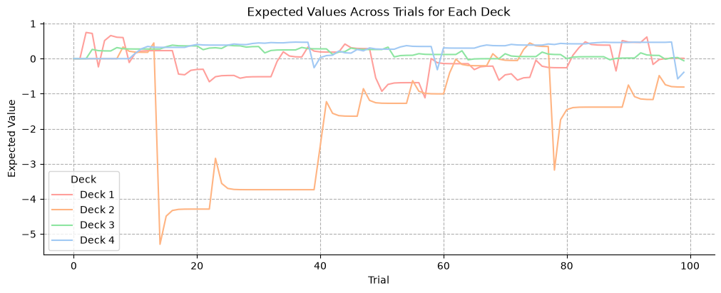
plot_data = pd.DataFrame(means_list, columns=["deck1", "deck2", "deck3", "deck4"])

# Use a seaborn color palette with softer colors
palette = sns.color_palette("pastel")

# Create a plot
plt.figure(figsize=(10, 4))

# Plot each deck as a separate line without markers and using the pastel palette
plt.plot(plot_data.index, plot_data["deck1"], color=palette[3], label="Deck 1")
plt.plot(plot_data.index, plot_data["deck2"], color=palette[1], label="Deck 2")
plt.plot(plot_data.index, plot_data["deck3"], color=palette[2], label="Deck 3")
plt.plot(plot_data.index, plot_data["deck4"], color=palette[0], label="Deck 4")

# Add titles and labels
plt.title("Expected Values Across Trials for Each Deck")
plt.xlabel("Trial")
plt.ylabel("Expected Value")

# Show legend
plt.legend(title="Deck")
plt.grid(linestyle="--")

sns.despine()

Bayesian inference

Using the responses simulated above, we can try to recover the value of the autoconnection strength. First, we start by creating the response function we want to optimize.

def response_function(autoconnection_strength, input_data, decisions, observed):
    """Log-probability of the decisions given the autoconnection strength.

    A fresh network is built on every call so the function stays pure (it does
    not mutate any shared state). This is what allows it to be wrapped with
    ``wrap_jax`` and differentiated during sampling.
    """
    # build the network, setting the autoconnection strength on the first level
    network = Network().add_nodes(kind="continuous-state", n_nodes=4, precision=5.0)
    for child in range(4):
        network = network.add_nodes(
            kind="continuous-state",
            value_children=child,
            tonic_volatility=tonic_volatility,
            precision=5.0,
            mean=0.0,
            autoconnection_strength=autoconnection_strength,
        )
    for parent_idx in range(4, 8):
        network = network.add_nodes(
            kind="continuous-state", value_children=parent_idx, precision=1.0
        )

    # run the model forward
    network = network.input_data(input_data=input_data, observed=observed)

    expected_means = jnp.stack(
        [network.node_trajectories[i]["expected_mean"] for i in range(4, 8)], axis=1
    )
    expected_variances = jnp.stack(
        [1.0 / network.node_trajectories[i]["expected_precision"] for i in range(4, 8)],
        axis=1,
    )

    x = 1.0 * expected_means + 1.0 * expected_variances  # (T, 4)
    x = x - jnp.max(x, axis=1, keepdims=True)  # normalize per row (per trial)
    decision_probabilities = jax.nn.softmax(x, axis=1)  # (T, 4)

    surprises = binary_surprise(x=decisions, expected_mean=decision_probabilities)
    surprises = jnp.where(surprises > 1e6, 1e6, surprises)
    surprise = surprises.sum()
    surprise = jnp.where(jnp.isnan(surprise), jnp.inf, surprise)

    return -surprise

Wrap the JAX log-probability function with wrap_jax so it can be used as a PyTensor Op during sampling. wrap_jax automatically provides both the forward evaluation and its gradient, so no custom Op has to be written by hand.

@wrap_jax
def hgf_logp(autoconnection_strength):
    """PyTensor-compatible log-probability wrapping the JAX response function.

    ``wrap_jax`` turns the JAX function into a PyTensor ``Op`` that provides both
    the forward evaluation and its gradient, so no custom ``Op`` is needed.
    """
    return response_function(
        autoconnection_strength,
        input_data=u,
        decisions=responses,
        observed=observed,
    )

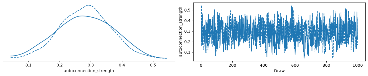
We are now ready to sample the model and estimate the value of autoconnection strength.

with pm.Model() as model:
    autoconnection_strength = pm.Beta("autoconnection_strength", 2, 2)
    pm.Potential(
        "hgf",
        hgf_logp(autoconnection_strength),
    )
    idata = pm.sample(chains=2, cores=1, backend="jax")

Initializing NUTS using jitter+adapt_diag...

Sequential sampling (2 chains in 1 job)

NUTS: [autoconnection_strength]

Sampling 2 chains for 1_000 tune and 1_000 draw iterations (2_000 + 2_000 draws total) took 3 seconds.

We recommend running at least 4 chains for robust computation of convergence diagnostics

az.plot_trace_dist(idata);

Parameter recovery

# Simulate one dataset per "participant", each generated with a different *true*
# autoconnection strength, and store every set of decisions in a single array.
tonic_volatility = -1.0
autoconnection_strengths = np.linspace(0.1, 0.9, 10)
n_participants = len(autoconnection_strengths)

responses = []
for true_autoconnection_strength in autoconnection_strengths:
    # build a network with the true autoconnection strength to simulate data
    simulation_network = Network().add_nodes(
        kind="continuous-state", n_nodes=4, precision=5.0
    )
    for child in range(4):
        simulation_network = simulation_network.add_nodes(
            kind="continuous-state",
            value_children=child,
            tonic_volatility=tonic_volatility,
            precision=5.0,
            mean=0.0,
            autoconnection_strength=true_autoconnection_strength,
        )
    for parent_idx in range(4, 8):
        simulation_network = simulation_network.add_nodes(
            kind="continuous-state", value_children=parent_idx, precision=1.0
        )

    simulation_network = simulation_network.create_belief_propagation_fn()
    attributes, edges, update_sequence = simulation_network.get_network()

    participant_responses = []
    for i in range(u.shape[0]):
        means = jnp.asarray([
            attributes[j]["expected_mean"] for j in range(4, 8)
        ]).ravel()
        variances = jnp.asarray([
            1 / attributes[j]["expected_precision"] for j in range(4, 8)
        ]).ravel()

        decision_probabilities = softmax(beta_1 * means + beta_2 * variances, axis=0)
        decision_probabilities = np.asarray(decision_probabilities, dtype=float).ravel()

        response = np.random.multinomial(n=1, pvals=decision_probabilities)
        participant_responses.append(response)

        # step the HGF forward one trial
        attributes, _ = beliefs_propagation(
            attributes=attributes,
            inputs=(u[i], response, np.ones(1), None),
            update_sequence=update_sequence,
            edges=edges,
            input_idxs=simulation_network.input_idxs,
        )

    responses.append(np.asarray(participant_responses))

# stack into a single (n_participants, n_trials, 4) array
responses = jnp.asarray(responses)
observed = responses

Rather than looping over the datasets and fitting them one by one, we store the decisions in a single array and fit every dataset in parallel. The log-probability of a single dataset is mapped over the participant axis with jax.vmap.

def participant_logp(autoconnection_strength, responses, observed):
    """Log-probability of a single participant's decisions."""
    return response_function(
        autoconnection_strength,
        input_data=u,
        decisions=responses,
        observed=observed,
    )


@wrap_jax
def recovery_logp(autoconnection_strength):
    """Total log-probability across all participants, evaluated in parallel.

    ``vmap`` applies :func:`participant_logp` to every participant at once, mapping
    over the per-participant autoconnection strengths and decisions.
    """
    return vmap(participant_logp)(autoconnection_strength, responses, observed).sum()


with pm.Model() as recovery_model:
    autoconnection_strength = pm.Beta(
        "autoconnection_strength", 1, 1, shape=n_participants
    )
    pm.Potential("hgf", recovery_logp(autoconnection_strength))
    recovery_idata = pm.sample(chains=2, cores=1, backend="jax")

Initializing NUTS using jitter+adapt_diag...

Sequential sampling (2 chains in 1 job)

NUTS: [autoconnection_strength]

Sampling 2 chains for 1_000 tune and 1_000 draw iterations (2_000 + 2_000 draws total) took 39 seconds.

We recommend running at least 4 chains for robust computation of convergence diagnostics

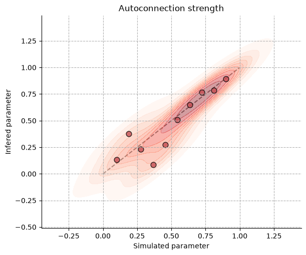
We can now visually inspect parameter recovery by plotting the simulated autoconnection strengths against the posterior means inferred for each dataset.

fig, ax = plt.subplots(figsize=(6, 5))

# ideal-recovery diagonal
ax.plot([0, 1], [0, 1], color="grey", linestyle="--", zorder=-1)

inferred_parameters = (
    recovery_idata
    .posterior["autoconnection_strength"]
    .mean(dim=("chain", "draw"))
    .values
)

sns.kdeplot(
    x=autoconnection_strengths,
    y=inferred_parameters,
    ax=ax,
    fill=True,
    cmap="Reds",
    alpha=0.4,
)
ax.scatter(
    autoconnection_strengths,
    inferred_parameters,
    s=60,
    alpha=0.8,
    edgecolors="k",
    color="#c44e52",
)

ax.grid(True, linestyle="--")
ax.set_xlabel("Simulated parameter")
ax.set_ylabel("Infered parameter")
ax.set_title("Autoconnection strength")
sns.despine()

System configuration

%load_ext watermark
%watermark -n -u -v -iv -w -p pyhgf,jax,jaxlib

Last updated: Tue, 16 Jun 2026

Python implementation: CPython
Python version       : 3.12.13
IPython version      : 9.14.1

pyhgf : 0.3.0
jax   : 0.4.31
jaxlib: 0.4.31

arviz     : 1.2.0
jax       : 0.4.31
matplotlib: 3.11.0
numpy     : 2.4.6
pandas    : 3.0.3
pyhgf     : 0.3.0
pymc      : 6.0.1
pytensor  : 3.0.7
scipy     : 1.17.1
seaborn   : 0.13.2

Watermark: 2.6.0