Hierarchical Bayesian modelling with probabilistic neural networks#
![]()
np.random.seed(123)
In the previous tutorials, we have fitted the binary, categorical and continuous Hierarchical Gaussian Filters (HGF) to observations to infer the values of specific parameters of the networks. proceeding this way, we were simulating computations occurring at the agent level (i.e. both the observations and actions were made by one agent, and we estimated the posterior density distribution of parameters for that agent). However, many situations in experimental neuroscience and computational psychiatry will require us to go one step further and to make inferences at the population level, therefore fitting many models at the same time and estimating the density distribution of hyper-priors (see for example case studies from [Lee and Wagenmakers, 2014]).
Luckily, we already have all the components in place to do that. We already used Bayesian networks in the previous sections when we were inferring the distribution of some parameters. Here, we only had one agent (i.e. one participant), and therefore did not need any hyperprior. We need to extend this approach a bit, and explicitly state that we want to fit many models (participants) simultaneously, and draw the values of some parameters from a hyper-prior (i.e. the group-level distribution).
But before we move forward, maybe it is worth clarifying some of the terminology we use, especially as, starting from now, many things are called networks but are pointing to different parts of the workflow. We can indeed distinguish two kinds:
The predictive coding neural networks. This is the kind of network that pyhgf is designed to handle (see Creating and manipulating networks of probabilistic nodes). Every HGF model is an instance of such a network.
The Bayesian (multilevel) network is the computational graph that is created with tools like pymc. This graph will represent the dependencies between our variables and the way they are transformed.
In this notebook, we are going to create the second type of network and incorporate many networks of the first type in it as custom distribution.
Simulate a dataset#
We start by simulating a dataset containing the decisions from a group of participants undergoing a standard one-armed bandit task. We use the same binary time series as a reference as the previous tutorials. This would represent the association between the stimuli and the outcome, the experimenter controls this and here we assume all participants are presented with the same sequence of association.
u, _ = load_data("binary")
Using the same reasoning as in the previous tutorial Using custom response models, we simulate the trajectories of beliefs from participants being presented with this sequence of observation. Here, we vary one parameter in the perceptual model, we assume that the tonic volatility (\(\omega\)) from the second level is sampled from a population distribution such as:
This produces belief trajectories that can be used to infer propensity for decision at each time point. Moreover, we will assume that the decision function incorporates the possibility of a bias in the link between the belief and the decision in the form of the inverse temperature parameter, such as:
Where \(A\) is a positive association between the stimulus and the outcome, \(\mu = \hat{\mu}_1^{(k)}\), the expected probability from the first level and \(t\) is the temperature parameter. We sample the temperature parameter from a log-normal distribution to ensure positivity such as:
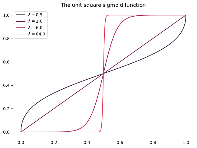
def sigmoid(x, temperature):
    """Compute the sigmoid response function with inverse temperature parameter."""
    return (x**temperature) / (x**temperature + (1 - x) ** temperature)
N = 10  # number of agents/participants in the study

# create just one default network - we will simply change the values of interest before fitting to save time
agent = Network().add_nodes(kind="binary-state").add_nodes(value_children=0)
# observations (always the same), simulated decisions, sample values for temperature and volatility
responses = []
for i in range(N):
    # sample one new value of the tonic volatility at the second level and fit to observations
    volatility = np.random.normal(-4.0, 1.0)
    agent.attributes[1]["tonic_volatility"] = volatility
    agent.input_data(input_data=u)

    # sample one value for the inverse temperature (here in log space) and simulate responses
    temperature = np.exp(np.random.normal(0.5, 0.5))
    p = sigmoid(x=agent.node_trajectories[0]["expected_mean"], temperature=temperature)

    # store observations and decisions separately
    responses.append(np.random.binomial(p=p, n=1))
responses = np.array(responses)
Group-level inference#
In this section, we start embedding the HGF in a multilevel model using PyMC. To fit many participants at once, we write the log-probability of a single participant as a JAX function (building the network with the Network class) and apply it to every participant in parallel using jax.vmap. The vectorized function is then exposed to PyMC with pytensor.wrap_jax, so it can be used inside a pm.CustomDist.
The per-participant parameters (here the tonic volatility and the inverse temperature) are passed as vectors whose first dimension is the number of participants, and the responses are stored as a 2D array of shape (n_participants, n_observations). The shared input sequence u is fixed, so it is captured once inside the log-probability function rather than being passed as a parameter.
```{note} Vectorizing over participants with vmap
To estimate group-level parameters, we fit many models at the same time - either on different input data, on the same data with different parameters, or on different datasets with different parameters. We achieve this by writing the log-probability for a single participant and mapping it over the participant axis with jax.vmap. Each mapped argument (tonic volatility, inverse temperature, responses) has the number of participants as its first dimension, so the n-th model uses the n-th value of every parameter and the n-th row of responses. Summing the resulting pointwise log-probabilities yields the total log-probability used by the custom distribution.
Hint
Observing the observer As we explained in the first part of the tutorials, probabilistic networks observe their environment through the inputs they receive and update beliefs using inversion of the generative model they assume for this environment. Here, we are taking a step back and want to use actions from agents that we assume are using such networks to make decisions to infer the values of some parameters from those networks. This is often referred to as observing the observer and this comes with a different concept of observations. Here, observations are the behaviours we can observe from the network and are directly influenced by the response model we define (i.e. how an agent uses its beliefs to act on the environment). The input data that are fed to the network are fixed, therefore we declare it when we create the HGF function compatible with PyTensor. The actions, or responses we get from the participant, are the things we want to explain using the PyMC model, therefor we treat it as observation in a custom distribution, a distribution that can simulate the behaviour of HGF networks under a set of parameters.
def participant_logp(tonic_volatility, inverse_temperature, responses):
    """Pointwise log-probability of a single participant's responses.

    Build a two-level binary HGF, feed it the (shared) input sequence `u` and
    return the log-probability of the participant's decisions under the binary
    softmax response model, one value per observation.

    The first time point reflects the network's initial (prior) state, before any
    observation has been processed, so its surprise does not depend on the
    parameters. We drop it here: it would otherwise add a constant offset to the
    total log-probability and, being constant across draws, break the
    leave-one-out cross-validation used for model comparison below.
    """
    surprise = (
        Network()
        .add_nodes(kind="binary-state")
        .add_nodes(value_children=0, tonic_volatility=tonic_volatility)
        .input_data(input_data=u)
        .surprise(
            response_function=binary_softmax_inverse_temperature,
            response_function_inputs=responses,
            response_function_parameters=inverse_temperature,
        )
    )
    return -surprise[1:]
@wrap_jax
def two_level_logp(value, tonic_volatility, inverse_temperature):
    """Total log-probability across all participants (a scalar).

    This is the log-probability function used by the PyMC custom distribution,
    so its first argument ``value`` is the observed responses (one row per
    participant). ``vmap`` applies :func:`participant_logp` to the ``N``
    participants in parallel - mapping over the per-participant tonic
    volatilities, inverse temperatures and responses - and the resulting
    pointwise log-probabilities are summed.
    """
    return vmap(participant_logp)(
        tonic_volatility.ravel(), inverse_temperature.ravel(), value
    ).sum()
Note
Pointwise log probabilities
The log-probability function used by the custom distribution returns the sum of the log-probabilities, which is all the sampler needs. Model comparison, on the other hand, requires pointwise estimates (one value per observation). Rather than recording them as a deterministic at every draw, we compute them once from the posterior samples after sampling (see the “Model comparison” section below), again reusing participant_logp through vmap.
with pm.Model() as two_levels_binary_hgf:
    # tonic volatility
    # ----------------
    mu_volatility = pm.Normal("mu_volatility", -5, 5)
    sigma_volatility = pm.HalfNormal("sigma_volatility", 10)
    volatility = pm.Normal(
        "volatility", mu=mu_volatility, sigma=sigma_volatility, shape=N
    )

    # inverse temperature
    # -------------------
    mu_temperature = pm.Normal("mu_temperature", 0, 2)
    sigma_temperature = pm.HalfNormal("sigma_temperature", 2)
    inverse_temperature = pm.LogNormal(
        "inverse_temperature", mu=mu_temperature, sigma=sigma_temperature, shape=N
    )

    # The multi-HGF distribution
    # --------------------------
    log_likelihood = pm.CustomDist(
        "log_likelihood",
        volatility,
        inverse_temperature,
        logp=two_level_logp,
        observed=responses,
    )
The multilevel model includes hyperpriors over the mean and standard deviation of both the inverse temperature and the tonic volatility of the second level.
Note
We are sampling the inverse temperature in log space to ensure it will always be higher than 0, while being able to use normal hyper-priors at the group level.
Sampling#
with two_levels_binary_hgf:
    two_level_hgf_idata = pm.sample(chains=2, cores=1, backend="jax")
Initializing NUTS using jitter+adapt_diag...
Sequential sampling (2 chains in 1 job)
NUTS: [mu_volatility, sigma_volatility, volatility, mu_temperature, sigma_temperature, inverse_temperature]
Sampling 2 chains for 1_000 tune and 1_000 draw iterations (2_000 + 2_000 draws total) took 50 seconds.
We recommend running at least 4 chains for robust computation of convergence diagnostics
# Compute the pointwise log-likelihood (one value per participant and observation)
# from the posterior samples, reusing `participant_logp`. We map over participants
# (inner vmap) and over posterior samples (outer vmap). Note that the first time
# point is dropped inside `participant_logp`, so there are `len(u) - 1` observations.
posterior = two_level_hgf_idata.posterior
volatility_samples = (
    posterior["volatility"].stack(sample=("chain", "draw")).transpose("sample", ...)
)
temperature_samples = (
    posterior["inverse_temperature"]
    .stack(sample=("chain", "draw"))
    .transpose("sample", ...)
)

pointwise_fn = vmap(
    vmap(participant_logp, in_axes=(0, 0, 0)),  # over participants
    in_axes=(0, 0, None),  # over posterior samples
)
pointwise = np.asarray(
    pointwise_fn(volatility_samples.values, temperature_samples.values, responses)
)  # shape (sample, participant, observation)

# reshape back to (chain, draw, participant, observation) and store as a
# `log_likelihood` group so it can be used for model comparison
n_chains = posterior.sizes["chain"]
n_draws = posterior.sizes["draw"]
n_observations = pointwise.shape[-1]
pointwise = pointwise.reshape(n_chains, n_draws, N, n_observations)
two_level_hgf_idata["log_likelihood"] = xr.Dataset({
    "log_likelihood": (
        ("chain", "draw", "participant", "observation"),
        pointwise,
    )
})
Visualization of the posterior distributions#
# Marginal posteriors of the group-level means, with the simulation values as
# reference lines.
pc = az.plot_dist(
    two_level_hgf_idata,
    var_names=["mu_temperature", "mu_volatility"],
)
for var_name, ref in {"mu_temperature": 0.5, "mu_volatility": -4.0}.items():
    pc.get_target(var_name, {}).axvline(ref, color="C1", linestyle="--")
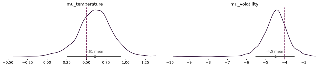
The reference values on both posterior distributions indicate the mean of the distribution used for simulation.
Model comparison#
The posterior samples we get from PyMC are crucial to inform inference over parameter values, but they can also be helpful to compare different models that were fitted on the same observations. Here, we use leave-one-out cross-validation [Vehtari et al., 2016], which is the default method recommended by Arviz. This function requires that the posterior samples also include pointwise estimates, it is therefore crucial to save this information during sampling, or alternativeæly to compute this manually from the samples a posteriori. We compute the expected log pointwise predictive density (ELPD) for one model, which indicates the quality of model fit (the higher the better). This quantity can be used to compare models side by side, provided that they are fitted to the same observed data.
%%capture --no-display
loo_hgf = az.loo(two_level_hgf_idata)
loo_hgf
Computed from 2000 posterior samples and 3190 observations log-likelihood matrix.

         Estimate       SE
elpd_loo -1677.26    25.65
p_loo       17.97        -

There has been a warning during the calculation. Please check the results.
------

Pareto k diagnostic values:
                         Count   Pct.
(-Inf, 0.70]   (good)     3187   99.9%
   (0.70, 1]   (bad)         2    0.1%
    (1, Inf)   (very bad)    1    0.0%
System configuration#
%load_ext watermark
%watermark -n -u -v -iv -w -p pyhgf,jax,jaxlib
Last updated: Tue, 16 Jun 2026

Python implementation: CPython
Python version       : 3.12.13
IPython version      : 9.14.1

pyhgf : 0.3.0
jax   : 0.4.31
jaxlib: 0.4.31

IPython   : 9.14.1
arviz     : 1.2.0
jax       : 0.4.31
matplotlib: 3.11.0
numpy     : 2.4.6
pyhgf     : 0.3.0
pymc      : 6.0.1
pytensor  : 3.0.7
seaborn   : 0.13.2
xarray    : 2026.4.0

Watermark: 2.6.0