pyhgf.plots.matplotlib.plot_nodes#

pyhgf.plots.matplotlib.plot_nodes(network, node_idxs, ci=True, show_surprise=True, show_posterior=False, figsize=(12, 5), color=None, axs=None)[source]#

Plot the trajectory of expected sufficient statistics of a set of nodes.

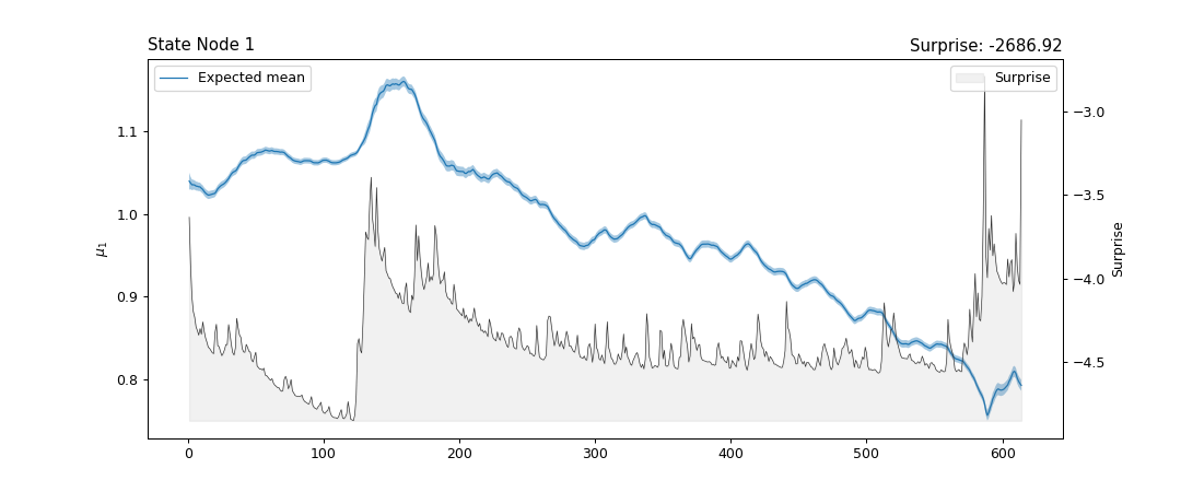
This function will plot the expected mean and precision (converted into standard deviation) before observation, and the Gaussian surprise after observation. If children_inputs is True, will also plot the children input (mean for value coupling and precision for volatility coupling).

Parameters:

network (Network) – An instance of main Network class.
node_idxs (int | list[int]) – The index(es) of the probabilistic node(s) that should be plotted. If multiple indexes are provided, multiple rows will be appended to the figure, one for each node.
ci (bool) – Whether to show the uncertainty around the values estimates (using the standard deviation \(\sqrt{\frac{1}{\hat{\pi}}}\)).
show_surprise (bool) – If True the surprise, defined as the negative log probability of the observation given the expectation, is plotted in the backgroud of the figure as grey shadded area.
show_posterior (bool) – If True, plot the posterior mean and precision on the top of expected mean and precision. Defaults to False.
figsize (tuple[int, int]) – The width and height of the figure. Defaults to (18, 9) for a two-level model, or to (18, 12) for a three-level model.
color (tuple | str | None) – The color of the main curve showing the beliefs trajectory.
axs (list | Axes | None) – A list of Matplotlib axes instances where to draw the trajectories. This should correspond to the number of nodes in the structure. The default is None (create a new figure).

Returns:

The Matplotlib axes instances where to plot the trajectories.

Return type:

axs

Examples

Visualization of nodes’ trajectories from a three-level continuous HGF model.

from pyhgf import load_data
from pyhgf.model import HGF

# Set up standard 3-level HGF for continuous inputs
hgf = HGF(
    n_levels=3,
    model_type="continuous",
    initial_mean={"1": 1.04, "2": 1.0, "3": 1.0},
    initial_precision={"1": 1e4, "2": 1e1, "3": 1e1},
    tonic_volatility={"1": -13.0, "2": -2.0, "3": -2.0},
    tonic_drift={"1": 0.0, "2": 0.0, "3": 0.0},
    volatility_coupling={"1": 1.0, "2": 1.0},
)

# Read USD-CHF data
timeserie = load_data("continuous")

# Feed input
hgf.input_data(input_data=timeserie)

# Plot
hgf.plot_nodes(node_idxs=1)

../../_images/pyhgf-plots-matplotlib-plot_nodes-1.png

pyhgf.plots.matplotlib.plot_nodes#

This Page